Recolorize & patternize workflow

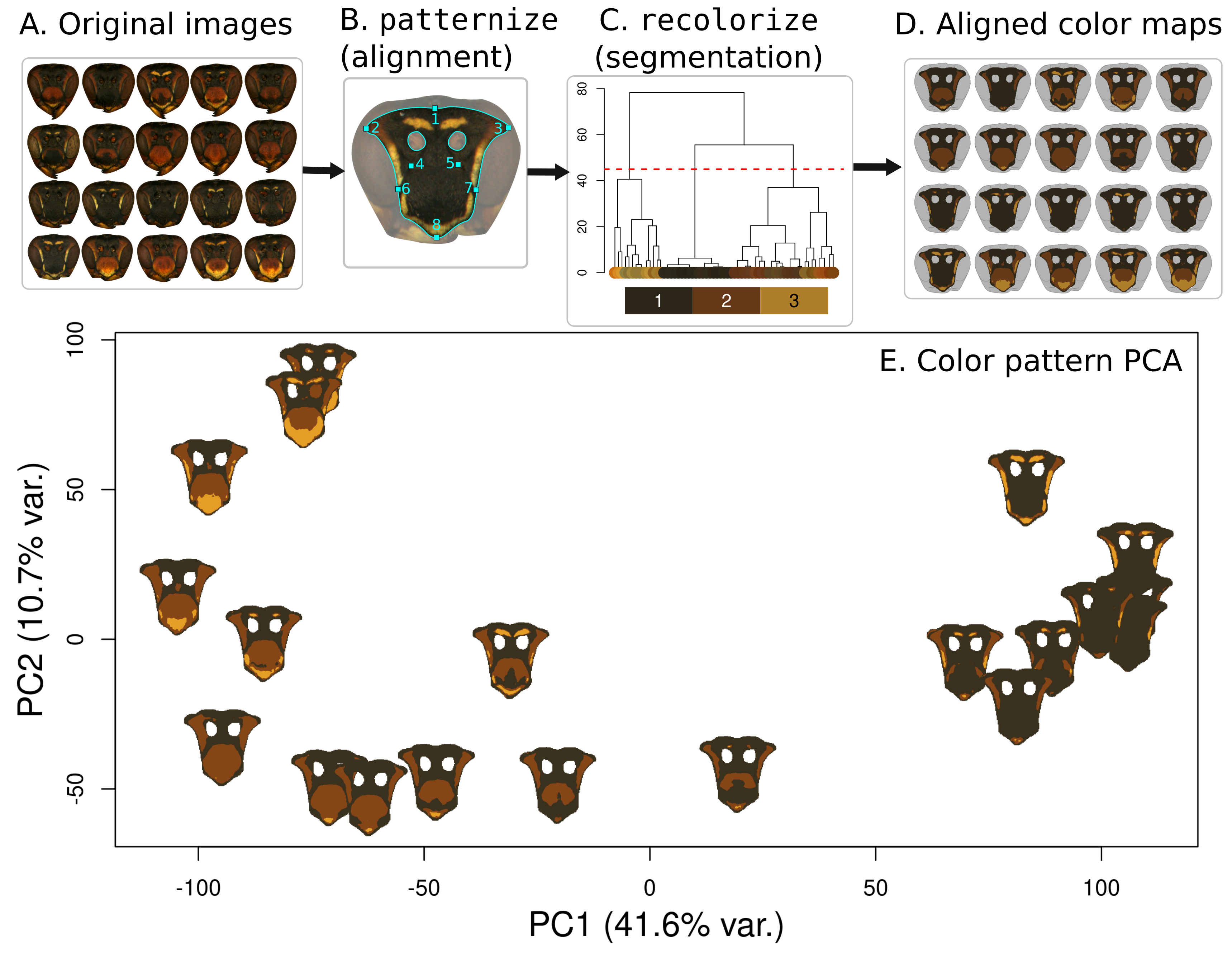
This tutorial will go through the process of combining patternize and recolorize tools to produce a PCA quantifying color pattern variation in wasp faces (Polistes fuscatus). This subset of 20 images (and workflow) is excerpted from ‘Evidence for a selective link between cooperation and individual recognition’ (Tumulty et al. 2023), with permission from the lead author. (Thanks James!)

The patternize package is an excellent tool for quantifying variation in color patterns. I use it frequently, because it’s a consistent, scaleable method for quantification that works for almost any organism, and it allows you to control for variation in shape, orientation, and size by first aligning all of your color patterns to a RasterStack—analogous to the Procrustes fit step of geometric morphometrics. It also helps that the package author, Steven Van Belleghem, is extremely friendly!

In practice, the most difficult step of using patternize is often the color segmentation: like several other color analysis packages and tools, patternize frequently relies on k-means clustering to extract color patches from images (especially for batch processing). That’s where recolorize comes in. In order to use recolorize to do the segmentation step for patternize, we have to follow three steps:

1. Align original images as RasterStacks using alignLan() in patternize
2. Segment the list of aligned images using recolorize
3. Convert list of segmented images back into the patternize format

Let’s do it!

Example files

All the data and code used in this tutorial can be found here in the ‘wasps’ subfolder: https://github.com/hiweller/recolorize_examples

Step 1: Image alignment in patternize

Note: Make sure you have installed the development version of patternize (e.g. by running devtools::install_github("StevenVB12/patternize")).

We’re starting with a folder of unaltered images of wasp faces. These images have been color-corrected and cropped to the wasp’s face, but the background hasn’t been masked out, since patternize will do that when we do the alignment.

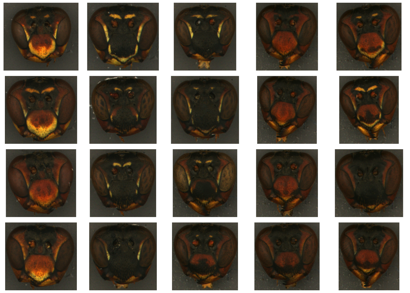
Note that even on this dataset—which is highly standardized—the images have slight variations in the size, shape, and angle of the head, making it difficult to differentiate variation due to color pattern differences from that due to other factors.

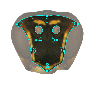
To use the alignLan() function, we need to provide XY coordinates of landmarks (one set per image). I did these in ImageJ using the multi-point tool, but really you just need a two-column, tab-delimited text file with X coordinates on the left and Y coordinates on the right, and no header. Our landmarking scheme for the wasp faces only had 8 points: So, I opened up each image in ImageJ, selected those landmarks using the multi-point tool, then saved those pixel coordinates as a plain text file with the same suffix. For example, the pixel coordinates for polistes_01.jpg is called polites_01_landmarks.txt (you can see it here).

I also made a mask for the images using the polygon selection tool in ImageJ, which will allow us to do the batch background masking. In this case, we only want to retain the frons and clypeus of the head (masking out the eyes and antennae openings), so I outlined them in a representative image (polistes_05) and saved those as XY coordinates as well (here). Because we’re aligning using landmarks, we only need to make one outline which will be applied to all images in the dataset—much faster than masking each image manually!

Once you have all those files (original images, XY landmark coordinates, and masking outline coordinates), we can combine them using patternize. I organized my files into separate folders (images in the original_images/ folder, landmark text files in the landmarks folder, etc), but you don’t have to do that so long as your files are organized and named in a way that works with the makeList() function.

# load library
library(patternize)

### Align set of 20 images ###

# set of specimen IDs
IDlist <- tools::file_path_sans_ext(dir("original_images/", ".jpg"))

# make list with images
imageList <- makeList(IDlist, type = "image",
                      prepath = "original_images/",
                      extension = ".jpg")

# make list with landmarks
landmarkList <- makeList(IDlist,
                         type = "landmark",
                         prepath = "landmarks/",
                         extension = "_landmarks.txt")

# Set target as polistes 05
target <- landmarkList[['polistes_05']]

# Set up mask, which excludes eyes/mandibles and antenna holes
mask1 <- read.table("masks/polistes_05_mask.txt", header = FALSE)
mask2 <- read.table("masks/polistes_05_Lantenna.txt", header = FALSE)
mask3 <- read.table("masks/polistes_05_Rantenna.txt", header = FALSE)

### Alignment ###
# this takes ~1 minute on a 16Gb RAM laptop running Ubuntu
imageList_aligned <- alignLan(imageList, landmarkList, transformRef = target, 
                              adjustCoords = TRUE,
                              plotTransformed = T, 
                              resampleFactor = 5, 
                              cartoonID = 'polistes_05',
                              maskOutline = list(mask1, mask2, mask3), 
                              inverse = list(FALSE, TRUE, TRUE))

The resulting imageList_aligned object is a list of aligned RasterBrick objects, one per image, with everything but the region of interest (frons and clypeus) removed.

Tip: I usually save this list as an .RDS file so I can load it back in at my convenience without having to do the alignment step again:

# save RDS file
saveRDS(imageList_aligned, "rds_files/imageList_aligned.rds")

# read it in:
imageList_aligned <- readRDS("rds_files/imageList_aligned.rds")

Step 2: Segment images in recolorize

The wonky step in this workflow is that patternize works with raster images, and recolorize works with arrays, so we have to convert from raster objects to arrays before using recolorize. The brick_to_array() function makes that fairly straightforward:

# load library
library(recolorize)

# convert from RasterBricks to image arrays using the brick_to_array function:
imgs <- lapply(imageList_aligned, brick_to_array)
names(imgs) <- names(imageList_aligned)

# save raster extents for later conversion:
extent_list <- lapply(imageList_aligned, raster::extent)

Now we have a list of image arrays. Plotting them using plotImageArray() helps us to see what the alignLan() step did for our original images:

(Note that it also flipped the images upside because the y coordinate systems are reversed–this is annoying, but doesn’t affect our results, so we’ll leave it for now.)

We want to map each of these wasp faces to the same set of three colors: dark brown, reddish brown, and yellow. K-means clustering could work in theory for this problem (we would fit n = 3 colors for each image), but in practice, we get the colors back in a random order—and they’re not actually the same color. Here’s what it looks like if we try to do that:

for (i in 1:length(imgs)) {
  rc <- recolorize(imgs[i], method = "k", n = 3, plotting = FALSE)
  plotColorPalette(rc$centers)
}

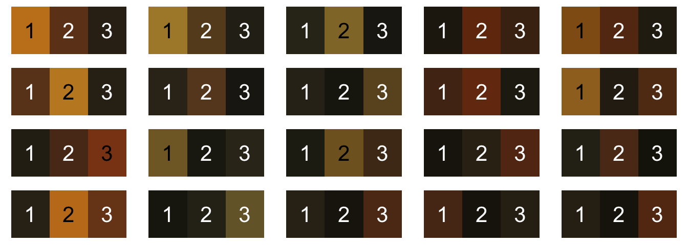
These colors are definitely similar across images, but they’re not consistent, especially since not all wasps have all three colors present. Maybe most intractably, they’re not in the same order: yellow is color 1, 2, or 3 depending on the image, and sometimes it’s not there at all.

Instead, we’ll come up with our list of 3 colors by combining color palettes across images, and then use the imposeColors() function in recolorize to map each of our images to the same color palette. First, generate a color palette for each image:

# make an empty list for storing the recolorize objects
rc_list <- vector("list", length(imgs))
names(rc_list) <- names(imgs)

# for every image, run the same recolorize2 function to fit a recolorize object:
for (i in 1:length(imgs)) {
  rc_list[[i]] <- recolorize2(imgs[[i]], bins = 3,
                              cutoff = 35, plotting = FALSE)
}

I kept it pretty simple for this example (we’re just calling recolorize2() with the same parameters for each image), but you could get more complicated with what you put in the for loop. (You could even choose to use k-means clustering as the method here by setting method = "k" and specifying the number of colors, since we’re just using it as a starting point, but since k-means is not deterministic that poses problems for repeatability.)

Next you can combine the color palettes from all of the recolorize objects in rc_list and use hclust_color to plot them and return a list of which colors to group together:

# get a dataframe of all colors:
all_palettes <- do.call(rbind, lapply(rc_list, function(i) i$centers))

# and for cluster sizes (as a proportion of their original image):
all_sizes <- do.call(c, lapply(rc_list, function(i) i$sizes))

# plot colors using hclust and return grouping list:
par(mar = rep(2, 4))
cluster_list <- hclust_color(all_palettes, n_final = 3)

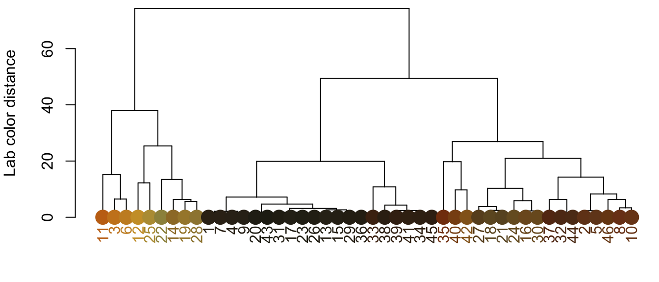
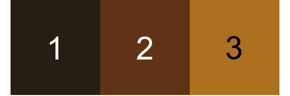
The cluster_list object is a list, each element of which is a vector of which of the original colors should be clustered together. See the rest of the hclust_color() options to various ways to combine colors by similarity—by default, it calculates the Euclidean distance matrix between all provided color centers in CIE Lab color space. We can use that list to combine all the colors and come up with our universal palette:

# make an empty matrix for storing the new palette
wasp_palette <- matrix(NA, ncol = 3, nrow = length(cluster_list))

# for every color in cluster_list...
for (i in 1:length(cluster_list)) {
  
  # get the center indices
  idx <- cluster_list[[i]]
  
  # get the average value for each channel, using cluster size to get a weighted average
  ctr <- apply(all_palettes, 2, 
                 function(j) weighted.mean(j[idx], 
                                           w = all_sizes[idx]))
  
  # store in the palette matrix
  wasp_palette[i, ] <- ctr
}

# check that our colors seem reasonable
par(mar = rep(0, 4))
plotColorPalette(wasp_palette)

And now, we can use imposeColors() to map every image to the same set of three colors:

impose_list <- lapply(imgs, function(i) imposeColors(i, wasp_palette, 
                                                     adjust_centers = FALSE, 
                                                     plotting = FALSE))

# let's look at our palettes!
layout(matrix(1:20, nrow = 4))
par(mar = rep(0, 4))
for (i in impose_list) {
  plotColorPalette(i$centers, i$sizes)
}

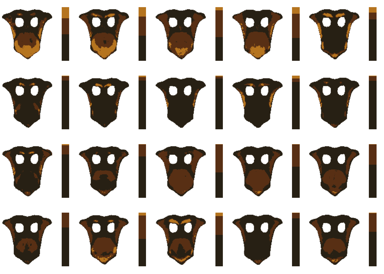
Although the proportions of each color vary by image, the order/value of the colors does not (unlike with k-means). This is the key step. As long as you can provide a color palette to which all of your images should be mapped, you can use imposeColors() to map every image to those colors. The earlier portion where we did an initial fit and used hclust_color is a good option when you want to come up with a color palette intrinsic to your original images, but it may still take some toying around before you find a palette that works.

The last step is to convert each recolorize fit in back to a patternize format, which we can do with the recolorize_to_patternize() function:

# convert to patternize:
patternize_list <- lapply(impose_list, recolorize_to_patternize)

# and set extents again:
for (i in 1:length(patternize_list)) {
  for (j in 1:length(patternize_list[[1]])) {
    raster::extent(patternize_list[[i]][[j]]) <- extent_list[[i]]
  }
}

This is a list of lists: there is one element per sample ID in patternize_list (20 total), and each of those elements is a list of RasterLayer objects, one per color class (3 per sample ID). You may need to reshuffle these depending on what you want to do.

Now, back to patternize!

Step 3: Color pattern analyses in patternize

Since we now have the images segmented in the way that patternize needs, we can run any of the regular patternize functions on it (see the methods paper and examples repository). Here, we’ll use a custom function based on code that Steven sent me for running a PCA on the entire color pattern (all three colors simultaneously, rather than one color class at a time). You can see the full function here. If you’ve downloaded the wasp example dataset, the easiest thing to do is to just source it and run the function on the list we made earlier:

source("patPCA_total.R")
wasp_pca <- patPCA_total(patternize_list, quietly = FALSE)

## Summing raster lists...

## Making dataframe from rasters...

## Running PCA on 3 colors and 20 images...

## done

That’s it! The wasp_pca object is a prcomp object (the standard class for principal components analysis in R).

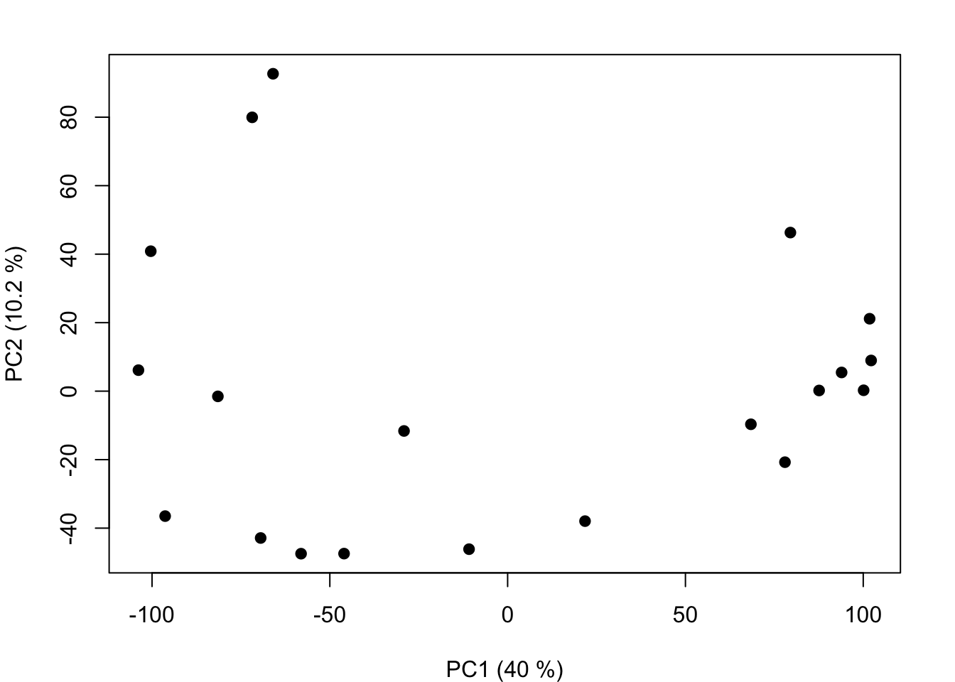
Bonus: visualization

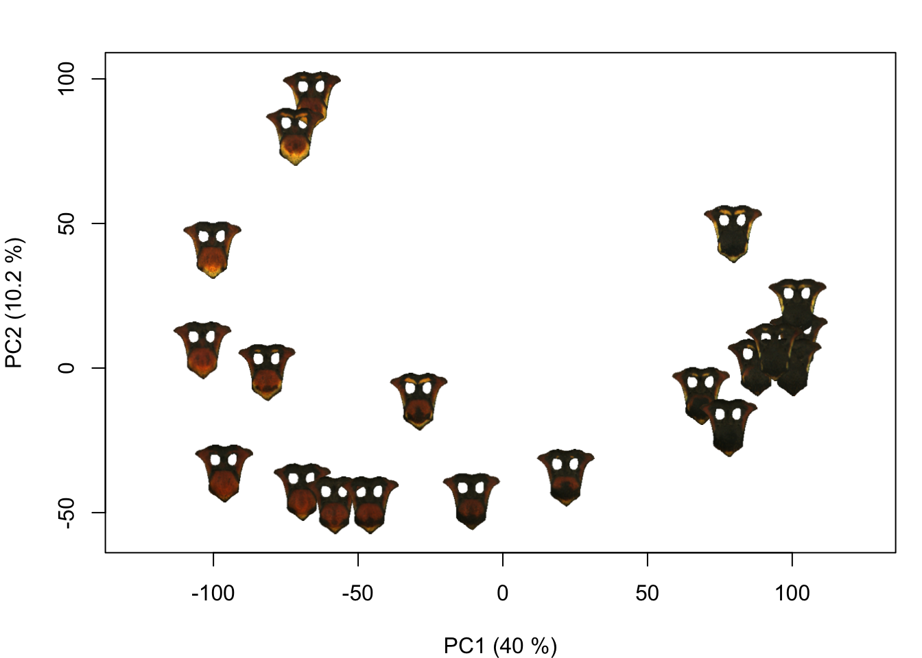
It can be hard to tell whether the PCA is capturing relevant axes of color pattern variation from a scatterplot; I find it more intuitive to plot some version the actual images. The add_image() function is an easy way to do that:

# first, make a blank plot
PCx <- 1; PCy <- 2
pca_summary <- summary(wasp_pca)
limits <- apply(wasp_pca$x[ , c(PCx, PCy)], 2, range)
par(mar = c(4, 4, 2, 1))
plot(wasp_pca$x[ , c(PCx, PCy)], type = "n",
     asp = 1,
     xlim = limits[ , 1] + c(-5, 5), 
     ylim = limits[ , 2] + c(-10, 10),
     xlab=paste0('PC1 (', round(pca_summary$importance[2, PCx]*100, 1), ' %)'),
     ylab=paste0('PC2 (', round(pca_summary$importance[2, PCy]*100, 1), ' %)'))

# then add images:
for (i in 1:length(impose_list)) {
  add_image(impose_list[[i]]$original_img, 
            x = wasp_pca$x[i, PCx],
            y = wasp_pca$x[i, PCy],
            width = 20)
}

You could also plot images from a folder on your computer:

plot(wasp_pca$x[ , c(PCx, PCy)], type = "n",
     asp = 1,
     xlim = limits[ , 1] + c(-5, 5), 
     ylim = limits[ , 2] + c(-10, 10),
     xlab=paste0('PC1 (', round(pca_summary$importance[2, PCx]*100, 1), ' %)'),
     ylab=paste0('PC2 (', round(pca_summary$importance[2, PCy]*100, 1), ' %)'))

# read in images from the original folder:
images <- lapply(dir("original_images/", full.names = TRUE),
                 readImage)

# and plot:
for (i in 1:length(images)) {
  add_image(images[[i]], 
            x = wasp_pca$x[i, PCx],
            y = wasp_pca$x[i, PCy],
            width = 20)
}

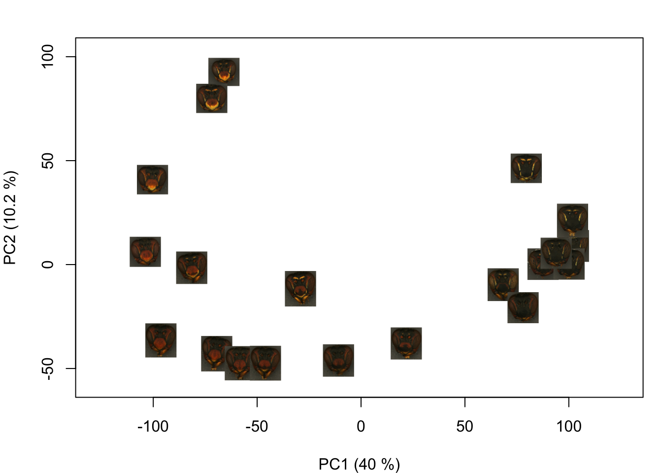(If I were to use these images for a paper figure, though, I would go through and mask out the background using transparencies—these are a little hard to see on a white background.)

That’s it for the tutorial. I would recommend downloading the example code and files from the linked GitHub repository if you want to try it out: there are a few steps involved, but ultimately it’s a reasonably simple procedure. I’d love to be able to write a one-and-done version of this process, but if you’ve been reading the other recolorize documentation, you’ll be familiar with my perspective on this. Basically, if I try to impose a general structure for how to do this every time, that’s not going to be flexible enough to encompass many use cases, and I prefer to keep things modular. Still, if you have any ideas for how to make this a more friendly process, I’m all ears!